Identifying Asset Pairs For Pairs Trading
Roadmap
Last time, we talked about how to identify stationary time series. Today we continue this line of thought by defining cointegration and looking at its usage in trading. In particular, we will discuss how a pairs trading strategy works.
Motivation
If we remember that stationarity assumes that a mean of a time series exist, we can conclude that if the time series wanders too far off its mean, it receives a pull back. Thus, the time series is mean reverting. If the time series is a series of prices, which is below its mean, we can conclude that it will rise back to its mean. So we can buy it and make profit by selling, if the price is back at its mean. The other way around, if the time series is above its mean, we can short the asset, and assuming mean reversion, we will make money in the long run.
Excursion: Continuous time
If you are familiar with stochastic processes, you may want to ponder the analogy to an Ornstein-Uhlenbeck process. An Ornstein-Uhlenbeck process is a stochastic process \(X_t\) which satisfies the following differential equation: \(\begin{align} dX_t = \theta (\mu-X_t)dt + \sigma dW_t \end{align}\) Here, \(\sigma\) is volatility, and \(W_t\) is Brownian motion. More interesting are the remining variables: \(\mu\) is the mean and \(\theta\) is an “elasticity coefficient”. The higher \(\theta\) is, the stronger is the pull towards the mean.
Pairs Trading
Unfortunately, simple mean reversion is hard to find. E.g. in stocks this would mean, that the company does not grow. But we may be able to construct a tradeable stationary time series. In a pairs trade the goal is to find two assets, such that a linear combination of the assets is stationary. In math that amounts to finding two time series \(X_t\) and \(Y_t\) such that a \(\beta\) exists with \(\begin{align} X_t = \beta Y_t + e_t \end{align}\) and the \(e_t\) stationary. If this holds, then the series \(X_t\) and \(Y_t\) are called cointegrated.
In the real world, that amounts to finding two companies which do
nearly the same, so the same economical factors apply. Two
companies which produce the same product and are in the same country
are affected by the same economical factors. But if one of them has a
failure in their supply chain, it may recover and thus we have a good
chance of a cointegrating relationship. A bunch of oil companies may
be a good pick. Or what about airlines.
Of course we could also go the other way, and scan random stocks for
cointegration. This will sometimes not work, since if we work with a
p-value of 5%, every 20th detected cointegration relationship will be
pure garbage.
How do we test cointegration?
If we knew the \(e_t\), then we could run an augmented dickey fuller test, like we did in the last post, but unfortunately, we do not know them. Thus, the traditional approach, also called the Engle-Granger two step method, is to first estimate the process \(e_t\) using, e.g., ordinary least squares and then testing \(e_t\) for stationarity.
Code
For this code I have set up a Jupyter notebook and converted it to markdown. If you are interested in toying around with the data yourself you can download the full notebook here. We test cointegration between the stock prices of Coca Cola and Pepsi, since they may be exposed to the same economical factors.
import pandas_datareader.data as web
import datetime
# We specify the timeframe and download the prices with Yahoo Finance
start = datetime.datetime(2011, 1, 1)
end = datetime.datetime(2014, 1, 27)
coke_prices = web.DataReader("KO", 'yahoo', start, end)
pepsi_prices = web.DataReader("PEP", 'yahoo', start, end)
Let us take a look at what we downloaded.
coke_prices.head()
| Open | High | Low | Close | Volume | Adj Close | |
|---|---|---|---|---|---|---|
| Date | ||||||
| 2011-01-03 | 65.879997 | 65.879997 | 65.110001 | 65.220001 | 18945600 | 27.033453 |
| 2011-01-04 | 65.019997 | 65.190002 | 63.810001 | 63.869999 | 27940400 | 26.473882 |
| 2011-01-05 | 63.790001 | 63.950001 | 62.860001 | 63.490002 | 34379000 | 26.316375 |
| 2011-01-06 | 63.619999 | 63.660000 | 62.830002 | 63.029999 | 21712400 | 26.125705 |
| 2011-01-07 | 62.779999 | 63.000000 | 62.560001 | 62.919998 | 16592800 | 26.080110 |
We are interested in the adjusted close. The close prices themselves do not work, because of stock splits.
coke_close=coke_prices['Adj Close']
pepsi_close=pepsi_prices['Adj Close']
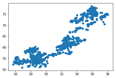
Let us do a scatterplot. If they are cointegrated, then we expect to see the points clustered around a line
import matplotlib.pyplot as plt
plt.scatter(coke_close, pepsi_close)
plt.show()
We fit a line with linear regression So pepsi = slope * coke + intercept + error
from scipy import stats
slope, intercept, r_value, p_value, std_err = stats.linregress(coke_close, pepsi_close)
print("slope: " + str(slope) +
      "\nintercept: " + str(intercept) +
      "\nr-value: " + str(r_value) +
      "\np-value: " + str(p_value) +
      "\nstd-err: " + str(std_err))
slope: 2.1868969195
intercept: -7.04139940461
r-value: 0.896540328487
p-value: 3.64783454604e-274
std-err: 0.0389638534876
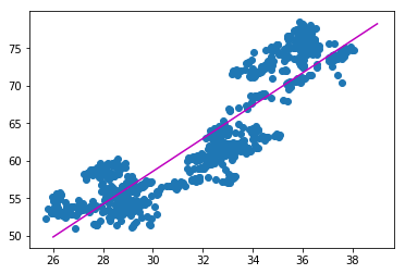
The p-value is small, which is good. Let us plot this thing with the fitted line
import matplotlib.pyplot as plt
plt.scatter(coke_close, pepsi_close)
x=[26,39]
plt.plot(x,[slope*x_i+intercept for x_i in x], color='m')
plt.show()
Now we compute the term e, which is the residue or the error term. If the error is stationary, then Coke and Pepsi are cointegrated.
error = pepsi_close - slope * coke_close - intercept
plt.plot(error)
plt.show()
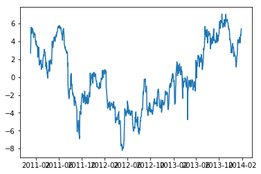
The plot looks okay, but it is not clear it if is really stationary. E.g., there is an upward trending segment in the middle. But we can test the error for stationarity.
import statsmodels.tsa.stattools as ts
ts.adfuller(error,1)
(-1.9345595231989032,
 0.31598188286172724,
 0,
 770,
 {'1%': -3.4388710830827125,
  '10%': -2.568772659807725,
  '5%': -2.8653008652386576},
 1257.1859133786406)
Remember the null hypothesis is, that there is a unit root. Having a unit root, means that the process is not stationary. The p-value is 0.31, so we cannot reject the null hypothesis.
Thus, Coke and Pepsi are not useful for pairs trading with the setup I described. There may be other setups, where it works. Maybe the timeframe is not useful. Maybe the error time series is not an AR(1)-process.
Let us take another example. There is an iShares MSCI Australia and an iShares MSCI Canada. These are two ETFs which track the economy of Australia, respectively Canada. Their ticker symbols are EWA and EWC. We will test their cointegration.
First, we define the timeframe and download the data from yahoo finance.
import pandas_datareader.data as web
import datetime

start = datetime.datetime(2003, 1, 1)
end = datetime.datetime(2008, 1, 27)
ewa_prices = web.DataReader("EWA", 'yahoo', start, end)
ewc_prices = web.DataReader("EWC", 'yahoo', start, end)
Again, we need to trade on the adjusted closes. Let us plot the two charts.
ewa_close=ewa_prices['Adj Close']
ewc_close=ewc_prices['Adj Close']

import matplotlib.pyplot as plt
ewa_close.plot(label='ewa', legend=True)
ewc_close.plot(label='ewc', legend=True)
plt.show()
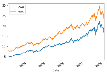
We can see that they have common jumps, so we can go on to the next step: drawing a scatterplot.
import matplotlib.pyplot as plt
plt.scatter(ewa_close, ewc_close)
plt.show()
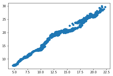
This fairly looks like a line. Perfect. So we fit a line.
from scipy import stats
slope, intercept, r_value, p_value, std_err = stats.linregress(ewa_close, ewc_close)
print("slope: " + str(slope) +
      "\nintercept: " + str(intercept) +
      "\nr-value: " + str(r_value) +
      "\np-value: " + str(p_value) +
      "\nstd-err: " + str(std_err))
slope: 1.27629111076
intercept: 1.79841662559
r-value: 0.989386266306
p-value: 0.0
std-err: 0.00525367636547
plt.scatter(ewa_close, ewc_close)
x=[4,22]
plt.plot(x,[slope*x_i+intercept for x_i in x], color='m')
plt.show()
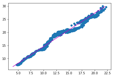
Looks great. Now we compute the error and test if it is mean-reverting.
error = ewc_close - slope * ewa_close - intercept
plt.plot(error)
plt.show()
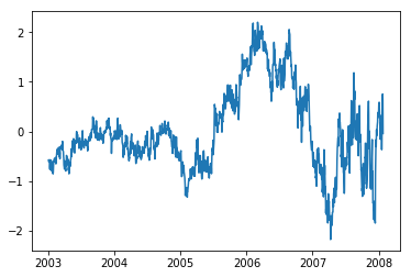
import statsmodels.tsa.stattools as ts
ts.adfuller(error,1)
(-3.3459094549609389,
 0.012946959495104054,
 1,
 1273,
 {'1%': -3.4354973175106842,
  '10%': -2.5679802172809003,
  '5%': -2.8638130956084464},
 -845.44796472685812)
We got a p-value of 0.0129. That means we are statistically significant. So we could go on to build a trading strat by trading on the error. The interesting part is that it is only significant, since I chose the timeframe appropriately. For other timeframes the cointegration relationship interestingly does not hold.