Backtesting With Zipline Ii

Introduction

In this post, we play again little bit around with python and the pandas-library. You may want to read the first part of this series. There we have backtested a simple crossing moving average strategy in pandas. We had a long/slow moving average over the last 40 days and a fast/short moving average over the last 20 days. When the stock price rockets skywards, the short moving average is above the long moving average. Then we will buy. If the short moving average crossed the long moving avergae again from above, we sold. If you remember, or if you have read the article again, we took most of the upturns but then sold too late.

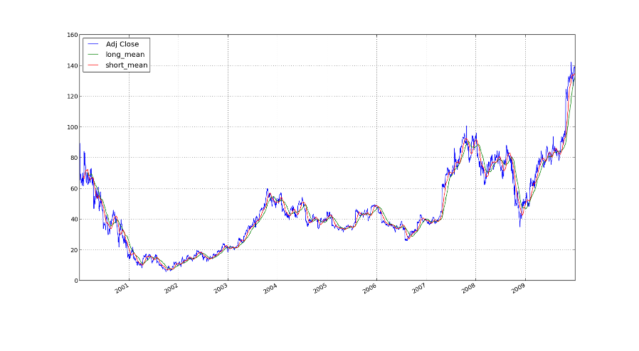
Here you have a nice image of the averages on the price of amazon stocks.

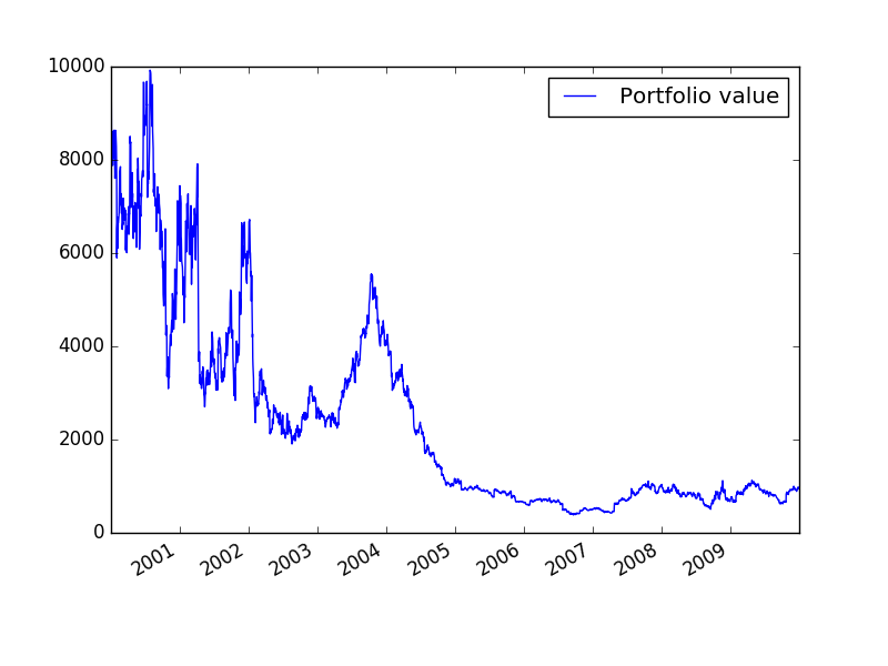
We reinvested everything back and plotted the returns which looked like the following.

So, how can we sell sooner and take all the money, so that we will be rich and bathing in gold like the mighty Dagobert Duck? Not so fast. First we will rewrite the strategy in zipline. This is an event-based framework for backtesting trading strategies. Last time we used pandas, which kind of sucked, since we could get into issues with look-ahead-bias. In zipline this is impossible. It works approximately like this: Each price change is fed to the trading algorithm as an event and the algorithm can decide what it wants to do. Thus it is slower, since it cannot compute the events in parallel, but on the other hand we will only trade on the old prices and not look into the future. Looking into the future leads to bugs you will never find and possibly also not even notice.

If we use zipline it will be easier to tweak with the algorithm later and, for example, set stoplosses to sell earlier.

The Code

The code is overly documented, since I do not really have experience with Zipline and so this may also serve as a reference for future programming adventures.
A zipline algorithm consists mainly of two functions: initialize and handle_data. initialize is called only once at the start of the trading algorithm. Here we need to setup everything. The function handle_data is executed at each bar. This is the event-based approach I mentioned earlier. Due to this it will be impossible to accidentally look into the future and introduce hard to find errors.

from zipline.api import record, symbol, order_target_percent
from zipline import run_algorithm
from datetime import datetime
import pytz

def initialize(context):
    """
    initialize is a function which is calld once at the start of the
    algorithm. The context is for maintaining state throughout
    multiple trading events.
    """
    context.amzn = symbol('AMZN')
    # Here we reference the amazon stock

def handle_data(context, data):
    """
    This function is called at the end of each trading bar.
    It takes the context and the data object.
    The data object contains the state of the current securities.
    """
    record(AMZN=data[context.amzn].price)
    # We record the price so we acn later track it.
    long_mavg = data.history(context.amzn, 'close', 41, '1d')[:-1].mean()
    # The long moving average is the mean of the prices of the last 40
    # days. In fact I take the last 41 days and throw the current day
    # away, since it is not finished.
    short_mavg = data.history(context.amzn, 'close', 21, '1d')[:-1].mean()
    # The short moving average is the mean of the prices of the last 20
    # days
    record(long_mavg=long_mavg)
    record(short_mavg=short_mavg)
    # We also record the two averages for later plotting
    if short_mavg > long_mavg:
        # If the short moving average is above the long moving average
        # we allocate 100% of our stock to AMZN
        if data.can_trade(context.amzn):
            # We need to check if the security is tradeable or if
            # trading is halted due to some event
            order_target_percent(context.amzn, 1.00)
    else:
        if data.can_trade(context.amzn):
            order_target_percent(context.amzn, -1.00)

# Set up the stuff for running the trading simulation
base_capital = 10000
start = datetime(2000, 1, 1, 0, 0, 0, 0, pytz.utc)
end = datetime(2010, 1, 1, 0, 0, 0, 0, pytz.utc)
# run the trading algorithm and save the results in perf
perf = run_algorithm(start, end, initialize, base_capital, handle_data,
        bundle = 'quantopian-quandl')

# Draw a nice plot of the value of our portfolio and save it
import matplotlib.pyplot as plt
plt.figure()
perf.portfolio_value.plot(label="Portfolio value")
# This is was generated by the run_algorithm
plt.legend()
plt.savefig('returns.png')

plt.figure()
perf.AMZN.plot(label='AMZN')
perf.long_mavg.plot(label='Long Moving Average')
perf.short_mavg.plot(label='Short Moving Average')
# These were recorded by the record function above
plt.legend()
plt.savefig('amzn.png')

If you run this code it will be confused as there are not data sources. To me it said:

ValueError: no data for bundle 'quantopian-quandl' on or before 2016-08-13 10:50:03.317389+00:00
maybe you need to run: $ zipline ingest quantopian-quandl

Though this suggestion did not work:

(venv) me@localhost:~$ zipline ingest quantopian-quandl
Usage: zipline ingest [OPTIONS]

Error: Got unexpected extra argument (quantopian-quandl)

Instead I had to run zipline ingest -b quantopian-quandl, to say that it is a bundle.

Results

Here is the resulting value of our portfolio:

and here the computations for the short and long moving average for debugging purposes:

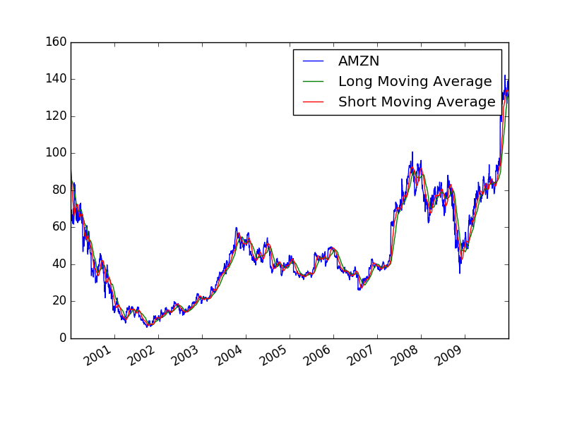
You can see that the stock values are like in our simulation with pandas. So we are not completely off the track.

You may notice that our portfolio on the other hand does not look at all like our previous result. This is due to multiple factors: First we have a much more realistic backtester. In zipline I check if AMZN is tradable at that day, which I did not do in pandas. Further Zipline also handles the Slippage. I do not get the orders filled immediately but instead my orders have an effect on the order book. Zipline simulates this and thus destroys our toy example even more. In the pandas simulation we got the trading data from Yahoo Finance, whereas now we get it from quandl.

An of course there may be simple programming mistakes. In particular I wonder why we do not have the plateaus anymore like in the previous

Addendum

I just realized that in the previous post we did not sell when the short moving average was below the long moving average. Instead we only liquidated the position. That explains the missing plateaus in the PnL graph.