Backtesting With Pandas

Introduction

In this post, we play a little bit around with python and the pandas-library. The motivation is the backtesting of algorithmic trading strategies. Suppose we know that market values are mean-reverting, i.e., they will always cross their average. Then we can implement a trading strategy based on that and get rich.
To be more specific, we buy, when the current market price goes above the average of the last \(k\) days and we sell if it falls below the average of the last \(k\) days. The problem is, that market prices contain a lot of noise, so we need to smooth the signal. We can do this by taking the average of the last \(t\) days, where \(t<k\). Taking the average over the last \(t\) days is called a moving average because we do it for every day.
The point of this post is to implement this strategy and test it against historical stock data of Amazon.

Let the fun start

First, we import pandas. That’s a library for working with time series and data munging.

In: import pandas as pd
In: import pandas.io.data
In: import datetime

Next we get ten years of historical data from amazon. Thanks to yahoo finance for their great API, which allows us to do this easily.

In: amzn=pd.io.data.get_data_yahoo('AMZN', start=datetime.datetime(2000,1,1), end=datetime.datetime(2010,1,1))
In: amzn.head()
Out: 
             Open   High    Low  Close    Volume  Adj Close
Date                                                       
2000-01-03  81.50  89.56  79.05  89.38  16117600      89.38
2000-01-04  85.38  91.50  81.75  81.94  17487400      81.94
2000-01-05  70.50  75.12  68.00  69.75  38457400      69.75
2000-01-06  71.31  72.69  64.00  65.56  18752000      65.56
2000-01-07  67.00  70.50  66.19  69.56  10505400      69.56

Seems to work. So what is this?
Open denotes the price in the morning, when the exchange opens.
Close denotes the price in the evening, when the exchange closes.
High is the highest price of this asset, which was achieved on this day.
Low is the lowest price of this asset, which was achieved on this day.
Volume is the traded volume, i.e., how much of the stock was traded on that particular day.
Adj Close denotes the adjusted closing price. This is mostly the same as the closing price, but takes into account events such as stock splits or dividends.
Why is the opening price of the current day not the same as the closing price of the previous day? During night, when the exchange is closed, orders keep coming in, but they do not get traded. So on the next day, when the exchange opens again, it computes a new opening price based on the overnight orders. I do not (yet?) know how that works exactly, so take my explanation with a grain of salt.

For evaluating our strategy we only use the adjusted close price, so we throw all this other stuff away.

In: amzn=amzn[['Adj Close']]
In: amzn.head()
Out: 
            Adj Close
Date                 
2000-01-03      89.38
2000-01-04      81.94
2000-01-05      69.75
2000-01-06      65.56
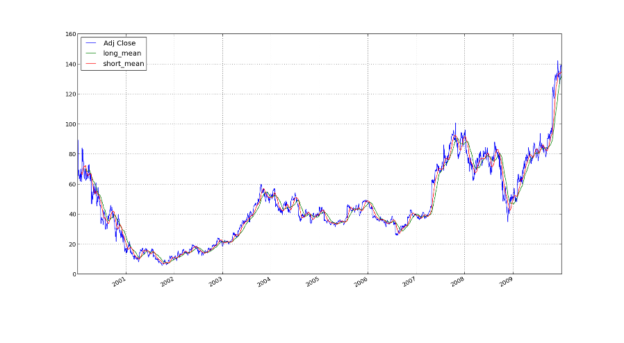
2000-01-07      69.56

We now compute some rolling means. We need two of them. A long one to capture the overall trend and a short one to smooth out the noise in the data. We let the short one be over 20 days and we take 40 for the long rolling average.

In: amzn['short_mean']=pd.rolling_mean(amzn['Adj Close'], 20)
In: amzn['long_mean']=pd.rolling_mean(amzn['Adj Close'], 40)

In: amzn.head(15)
Out: 
            Adj Close  short_mean  long_mean
Date                                        
2000-01-03      89.38         NaN        NaN
2000-01-04      81.94         NaN        NaN
2000-01-05      69.75         NaN        NaN
2000-01-06      65.56         NaN        NaN
2000-01-07      69.56         NaN        NaN
2000-01-10      69.19         NaN        NaN
2000-01-11      66.75         NaN        NaN
2000-01-12      63.56         NaN        NaN
2000-01-13      65.94         NaN        NaN
2000-01-14      64.25      70.588        NaN
2000-01-18      64.12      68.062        NaN
2000-01-19      66.81      66.549        NaN
2000-01-20      64.75      66.049        NaN
2000-01-21      62.06      65.699        NaN
2000-01-24      70.12      65.755        NaN

The problem of the moving averages is that not only do they smooth the signal and remove the noise, but they also add latency as you can see above. The computation of short_mean, the moving average over the last 20 days, can only be computed if we have 20 days before it. That is why you see NaN, not a number, above.
In general adding latecy is bad, because then some trends are over, before they are even noticed. To understand this, let us draw a picture.

In: import matplotlib as mpl
In: import matplotlib.pyplot as plt

In: amzn.plot()
In: plt.show()

For your convenience, I have embedded the thing here:

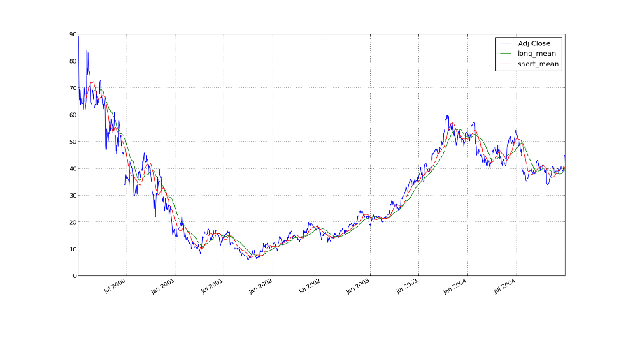
I have also made a version only over the last five years to make the time lag more clear.

If the short moving average is now above the long moving average, then we are on a short-term upwards trend. At least that is the theory. That means, that we will buy. If the averages cross the other way around, we sell. Otherwise we do nothing.

In: amzn['order']=0
In: amzn['order'][amzn.short_mean>amzn.long_mean]=1
In: amzn['order']=amzn['order'].shift(1)

This means that we make a new column which consists of a one if the short moving average is above the long moving average, otherwise it contains a zero. The shift in the last line is, because we compute on the closing prices. That means that we will then buy/sell on the next day, so we shift the buying signal one day.

Now we need to calculate our relative returns for each day:
\(r_t = \frac{p_t - p_{t-1}}{p_{t-1}} = \frac{p_t}{p_{t-1}} - 1\)

In: amzn['returns']=amzn['Adj Close'] / amzn['Adj Close'].shift(1) - 1
In: amzn.head()
Out: 
            Adj Close  short_mean  long_mean  order   returns
Date                                                         
2000-01-03      89.38         NaN        NaN    NaN       NaN
2000-01-04      81.94         NaN        NaN      0 -0.083240
2000-01-05      69.75         NaN        NaN      0 -0.148767
2000-01-06      65.56         NaN        NaN      0 -0.060072
2000-01-07      69.56         NaN        NaN      0  0.061013

We have only returns when we trade. That means that we multiply the returns with the buying signal.

In: amzn['returns']=amzn['returns']*amzn['order']
In: amzn.head()
Out: 
            Adj Close  short_mean  long_mean  order  returns
Date                                                        
2000-01-03      89.38         NaN        NaN    NaN      NaN
2000-01-04      81.94         NaN        NaN      0       -0
2000-01-05      69.75         NaN        NaN      0       -0
2000-01-06      65.56         NaN        NaN      0       -0
2000-01-07      69.56         NaN        NaN      0        0

If you have not yet worked extensively with numerical algorithms I should perhaps explain the -0. We are working with floating point arithmetic, so we naturally have rounding errors. So, a zero in the computer can be just a very small number. If this is negative, then python says -0. If you are more interested, then google for “floating point arithmetic” or search for some introductory lecture notes about numerical algorithms.

Since we reinvest all returns, we need to take a cumulative product over the last column.
\(i_t = (i_{t-1} + i_{t-1} \cdot r_t) = (1 + r_t) \cdot i_{t-1}, \quad i_0 = 1\)

In: amzn['cumreturns']=(1+amzn.returns).cumprod()
In: amzn.head()
Out: 
            Adj Close  short_mean  long_mean  order  returns  cumreturns
Date                                                                    
2000-01-03      89.38         NaN        NaN    NaN      NaN         NaN
2000-01-04      81.94         NaN        NaN      0       -0           1
2000-01-05      69.75         NaN        NaN      0       -0           1
2000-01-06      65.56         NaN        NaN      0       -0           1
2000-01-07      69.56         NaN        NaN      0        0           1

Now we are nearly finished. In the last column, cumreturns, we have the cumulative returns. We can now plot it and see if it looks good.

In: amzn.cumreturns.plot()
Out: <matplotlib.axes.AxesSubplot at 0x5fe40d0>
In: plt.show()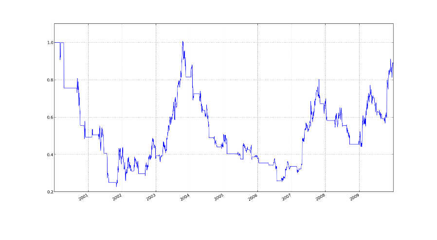

As we can see, the buying order nearly always starts on an upwards trend. That is good. The problem is that we sell too late. This is perhaps due to the time lag which we have introduced by taking all those moving averages. If we take into account other stuff like transactions costs this strategy is not profitable but was fun to code and play with nevertheless.

Improvements

Why did we take a moving average over 20 days and another one over 40 days? Why not 10 and 20 days? I do not know. This was just to play around. In general we can take an average over \(t\) and \(k\) days. Then we can view the returns as a function in terms of \(k\) and \(t\). Let us call it \(r(k,t)\). We can now maximize this thing with a numerical method of your choice.
The problem is, that we have a curve-fitting bias. The optimal \(k\) and \(t\) would be only optimal for this particular curve. For future prices, other parameters would be a better fit.

I currently do not see how we can avoid overfitting. There are things called stop-loss and take-profit which could possibly help.
Stop-loss means, that if we have some stocks and the price falls below the stop-loss, then we sell them automatically. The stop-loss is thus a threshhold to bound the losses.
Take-profit is the same but in the other direction. Take-profit would yield an upper bound on the profit. I think that this would make sense in our scenario, since according to the chart, we sell too late. Take-profit would close the trade earlier.
But with stop-loss, as well as with take-profit, we have introduced more parameters, which we need to choose carefully.

Since this section is called improvements, i should also mention that for a realistic model, we need to accommodate the transaction fees and slippage. Slippage means, that if we place a big buy order, the market price goes up and we need to pay a little bit more than planned. That is a very simplified explanation, but it captures the core idea. Including slippage in this model is difficult, because we compute on historical data, so we cannot take into account our own feedback back into the market.

Thanks

Thanks to twiecki, from whom I have borrowed some formulas and pythonic design ideas.