Intro

Today I want to write about Bayesian statistics. Bayesian statistics is an approach to inferring probabilities. It provides ways to specify a previous belief (the prior) and update the belief, as new observations are made and new data becomes available. Thus, it is a valuable instrument for very diverse areas such as earth quake prediction or clinical trials.

Previously, Bayesian analysis was often cumbersome, as the involved probabilities are often hard to compute. In most cases, the equations are not solvable analytically at all. However, in the last few years new algorithms such as Hamiltonian Monte Carlo or NUTS have been discovered that enable to tackle the math part. As a consequence, it was possible to design probabilistic programming languages such as Stan or PyMC3 that separate the math from the modelling. It is now possible to handle the occurring probability distributions without explicitly handling the math parts.

In this blog post, I contrast Bayesian analysis with machine learning and the frequentist interpretation of probability. Then, I explain Bayes’ theorem, the heart of Bayesian analysis. I conclude with an example of contemporary usage of Bayesian analysis by inferring the probability of a biased coin with PyMC3.

Bayesian Modelling vs Machine Learning

Machine learning is usually concerned with predicting future behavior based on observed data. This can encompass classifying or clustering data.

As an example, machine learning software can classify the gender of persons based on their facial features. For this, the machine learning algorithm is trained on a data set of facial images, together with the annotated gender. In a subsequent phase, the algorithm can associate novel facial images, which were not previously in the data set, to a gender.

One main drawback in my personal point of view is the limited introspection of machine learning. No additional knowledge is created that explains why the model works the way it does. In our example, if an image is assigned to the wrong gender, there are only very limited ways to trace the origins of this failure.

Further, the lack of transparency within the algorithm can lead to algorithmic bias. If the training set lacks people of color or of nonbinary genders, the algorithm will fail on those groups.

Bayesian modelling, in contrast to machine learning, is not focussed on predicting, but instead on inferring. In Bayesian modelling, the internal parameters of the model are inferred based on the observed data. This helps significantly in understanding the data and the process that generates the data. However, in Bayesian modelling a model needs to be crafted by hand, in contrast to machine learning, where the algorithm can learn the model by itself.

Bayesian vs Frequentist Interpretations of Probability

Whenever I read a general introduction to Bayesian methods, the author contrasts it with frequentist approaches to probability. It took me a long time to understand the practical implications of this distinction. So, if you do not grasp this, do not despair. This stuff is hard.

There are two main philosophical interpretations of probabilities: the frequentist and the Bayesian interpretation.

In the frequentist interpretation, probability is based on the frequency of how often something has already been observed. If a coin is flipped 10 times and lands on head 3 times and on tail 7 times, then the probability of the coin landing on head is 30%. From a frequentist perspective it does not make sense to talk about probabilities of things that can not be repeated.

In the Bayesian interpretation, probability is based on the certainty, sometimes also called the belief, of an observation happening. This allows to talk about the probability of life on mars, or the probability of some person being elected as president. In contrast, from a frequentist point, either there is life on mars, or there is no life on mars, but there is no way to talk about the certainty.

In particular, when a coin is thrown ten times and lands on head 3 times or when a coin is thrown 100 times and lands on head 30 times, there is no difference in the frequentist interpretation. A frequentist will in both cases infer that the probability of the coin landing on head is 30%, as that is the maximum likelihood estimator. In a Bayesian setting, however, the certainty of the coin landing on heads 30% of the time can be estimated. Or in other words, the probability of the coin landing on heads is not only a single number, but comes from a probability distribution.

Bayes’ Theorem and Challenges

Let us now come to the heart of Bayesian analysis: Bayes’ Theorem. Bayes’ theorem is a simple formula that allows the updating of a belief when new data is made available. Let us call \(D\) the observed data, \(\theta\) is a parameter of our model, \(P\) denotes the probability. Then Bayes’ theorem looks as follows:

This formula is not magical and can be derived from basic probability theory. However, Bayes’ theorem is very important and if you understand this formula well enough, then all books about Bayesian analysis are just footnotes to this formula. In fact this formula is so central, that each of the occurring terms has a special name.

• \(P(\theta \mid D)\) is called the posterior. It is the refined belief in \(\theta\) considering the available data \(D\).
• \(P(D\mid \theta)\) is called the likelihood. It is the probability of getting the data \(D\) when we use the parameter \(\theta\) in our model.
• \(P(\theta)\) is called the prior. This is the strength of our belief in \(\theta\) without considering any data.
• \(P(D)\) is called the evidence. It is the least important part of the formula and often only considered as a normalizing factor, so that the sum of all probabilities is 1. If you want to actually compute this, you have to sum (or integrate) over all possible values of \(\theta\), weighted by their certainty.

If you want to take a look at an easy example of applying Bayes’ theorem, you can read one of my first blog posts.

One of the main problems when using Bayes’ theorem is that the formulas that occur are often not solvable analytically. Thus, for a long time, Bayesian analysis was limited to the usage of conjugate priors. These are prior distributions for a fixed likelihood, such that the posterior is again from the same family of distributions. As an example, the beta distribution is a conjugate prior for the likelihood function of the binomial distribution. This allows to update the posterior further, as even more new data becomes available.

Probabilistic Programming – An Example

In this section I will walk you through applying Bayesian modelling to a coin flip. We start with a coin that has an unknown probability \(\theta\) of landing on head. Thus, as prior distribution all probabilities are equally likely. The coin may fall on head with a probability of 30%, or 90% or something else. We do not know in advance. Thus, \(\theta\) is not treated as a single value (as in a frequentist setting) but instead as a random value itself.

This is modelled with a beta distribution. A beta distribution is a fancy distribution that has two parameters, \(\alpha\) and \(\beta\). Depending on their values, the beta distribution can take a wide variety of forms and thus is flexible enough for our purpose. For \(\alpha=\beta=1\) we get the uniform distribution. This is what we choose initially, as we think that all values of the bias \(\theta\) of the coin have the same probability.

A small but important detail is that we implicitly assume that the coin flips are independent, i.e., the probability of the coin landing on head does not change. Without this, the math would not work out. In our case it is a reasonable assumption, but keep it in mind, if you want to generalize this model.

Next, we need to acquire data to refine our estimation of \(\theta\). For this we throw the coin 10 times and count the number of heads. This follows a binomial distribution. As a nice fact, the beta distribution is a conjugate prior for the binomial distribution, thus further justifying our choice of distributions.

Using Bayes formula, we calculate the posterior, given the data of the coin flips. That means, we infer the probability of the coin landing on head, given some coin flips.

Even though this is a very simple example and can be solved analytically as we are in the beta-binomial model, it is not easy to calculate. And in fact, we will not compute this analytically, but rather use probabilistic programming for inferring the posterior probability. You can find the analytic solution in many introductory books to Bayesian statistics and in some blog posts. Note that the analytic solution is only “simple” to calculate, due to the fact that the beta distribution is a conjugate prior for the binomial distribution. In other cases, this cannot be computed analytically at all.

In mathematical notation, our model looks as follows:

The parameter \(\theta\) is the probability of the coin landing on head. \(y\) is the number the coin lands on head, given 10 flips of the coin.

First, we need to simulate the data of our coin flip, as i do not have a real biased coin at hand.

import numpy as np
from scipy import stats

np.random.seed(1)
N = 10
theta_real = 0.3 # this is unknown
data = stats.bernoulli.rvs(p=theta_real, size=N)

The coin flips in the array data are [0 1 0 0 0 0 0 0 0 0]. I have fixed the seed, so you can follow along at home in front of your screen.

Next, we compute the posterior, i.e., the probability distribution of \(\theta\), given access to the data. For this we use PyMc3, as it provides us with state of the art MCMC algorithms, so we do not have to care about the math.

import pymc3 as pm

with pm.Model() as my_model:
    theta = pm.Beta('theta', alpha=1, beta=1)
    y = pm.Bernoulli('y', p=theta, observed=data)
    trace = pm.sample(2000, random_seed=1)

Internally, the sample command is the part where all the magic happens. It uses the NUTS (No U-turn Sampler) which is an extension of the Hamiltonian Monte Carlo algorithm. But we do not have to care about that. All we have to care about is the correct modelling. PyMC3 will do its magic and give us a posterior.

Next, we want to visualize the posterior in order to evaluate it. For this, we are using the plot_posterior function from ArViz.

import arviz as az
import matplotlib.pyplot as plt

az.plot_posterior(trace)
plt.show()

This yields the following image.

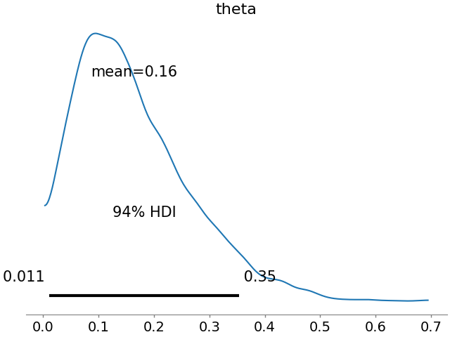
This is the approximation of the posterior probability of \(\theta\). The peak is at 0.16 as we only had one head among the ten throws of the coin. In a frequentist analysis, we would get 0.1 as the estimate, i.e., the mode of the Bayesian prior. However, in a Bayesian analysis, we get the whole distribution of \(\theta\) and thus, our certainty.

I do not know with certainty (bad pun intended), why there is the difference between 0.16 and 0.1. I suspect it is due to the number of samples or some approximation error in the algorithm.

At the bottom we see the 94% HDI. This is the highest density interval (HDI) – a measure of dispersion of our distribution. It means that the real value of \(\theta\) is between 0.011 and 0.35 with a probability of 94%. The HDI is analogous to the confidence interval in frequentist statistics.

If we have more samples from the data, our estimate of the bias \(\theta\) is more exact and will converge to the real value of theta as you hopefully have guessed. Let us try the same Bayesian inference with more samples.

import numpy as np
from scipy import stats

np.random.seed(1)
N = 1000 # more samples this time.
theta_real = 0.3 # this is unknown
data = stats.bernoulli.rvs(p=theta_real, size=N)

import pymc3 as pm
import arviz as az
import matplotlib.pyplot as plt

with pm.Model() as my_model:
    theta = pm.Beta('theta', alpha=1, beta=1)
    y = pm.Bernoulli('y', p=theta, observed=data)
    trace = pm.sample(2000, random_seed=1)

az.plot_posterior(trace)
plt.show()

And we get the following estimation of the bias \(\theta\) of the coin.

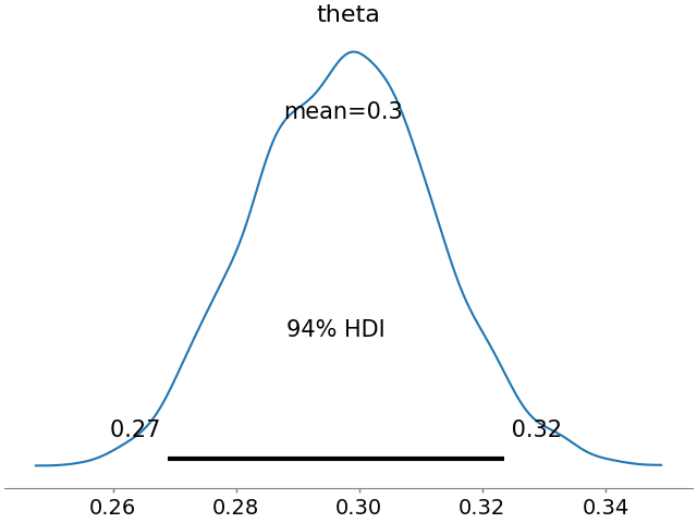
As you can see, the 94% HDI is now from 0.27 to 0.32 and the mean is 0.3.

Conclusion

As you have seen, making use of Bayesian models without a detailed understanding the math and algorithms behind it is not very hard. It is possible to build tailored Bayesian models that allow to infer information about the data and thus gain more insight than usual machine learning models.

I hope I could inspire you to go out and play around with that knowledge. Do not be intimidated if something breaks. That is part of learning.