Random Variables Without Expected Value

Introduction

In some of the last posts I wrote that some formula should give us the mean of a random variable “if it exists”. In this post I am going to introduce an example, where an intuitive approach of computing the expected value of a random variable does not work. You can also read this post as some statistics, if you substitute every ocurrence of “expected value” by “mean”.

Gaussian Distribution

Suppose we want to compute the average weight of stuff on my desk. How would you do that? We will take samples and weight them. The average of the weight of the samples should converge to the expected value of the weight of stuff on my desk. So we will take something and weight it. Suppose it weighs \(x_1\). Then we take another thing and weigh it. Suppose it weighs \(x_2\). And so on. Then, we will compute \begin{equation} \frac{1}{n}\sum\limits_{k=0}^n x_k \end{equation} This should be our expected weight for large enough \(n\).

In fact, I let you in on a little secret. The weight of the stuff on my desk has a gaussian distribution with mean \(0\). Yes, I have some anti-matter on my table. So we can write python and produce a nice plot.

import numpy as np

import matplotlib as mpl
import matplotlib.pyplot as plt

weights=np.random.randn(100)
plt.plot(weights.cumsum()/range(1,101))
plt.show()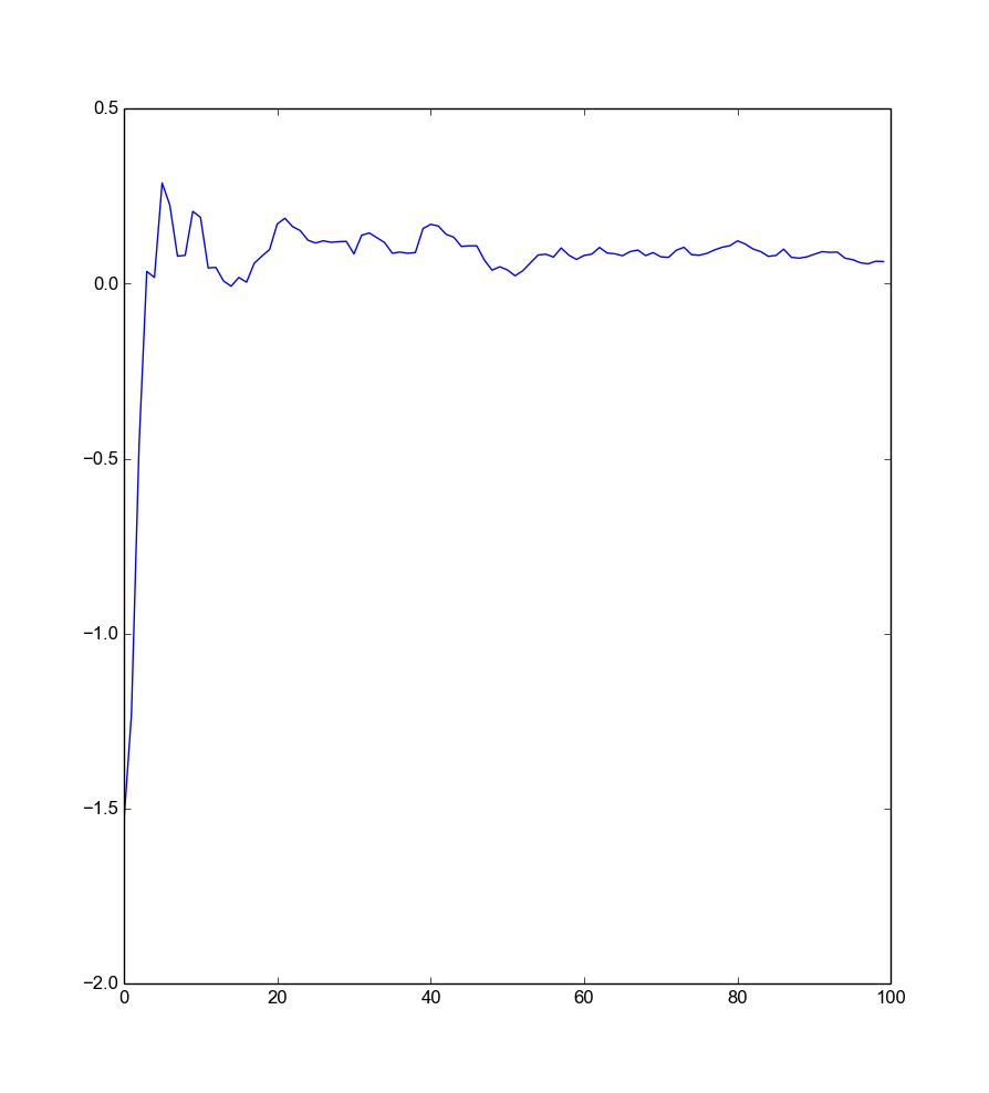

As you can see, the first item has a very negative weight, but in the end its influence fades as we weight more other stuff. So the approach works. At least this time. You can see that the expected value approaches \(0\).

Cauchy Distribution

The stuff on the table on my colleague is more interesting. Let us suppose that if we take a sample from his table this is akin to taking two normally distributed variables and dividing them. We can again produce a nice plot of the averages of the stuff we have sampled:

import numpy as np

import matplotlib as mpl
import matplotlib.pyplot as plt

weights=np.random.randn(100)/np.random.randn(100)
plt.plot(weights.cumsum()/range(1,101))
plt.show()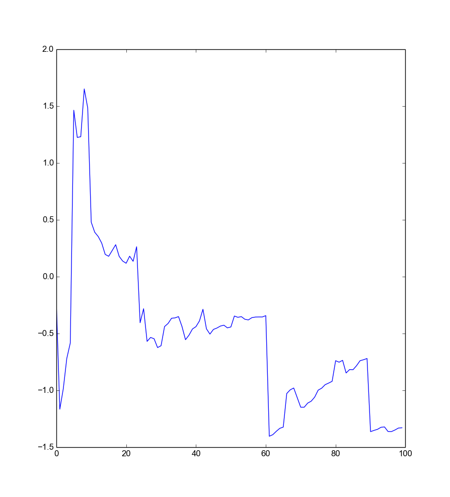

Hmm… not sure if that converges. Perhaps we have not yet enough samples. Let us take \(10000\).

weights=np.random.randn(10000)/np.random.randn(10000)
plt.plot(weights.cumsum()/range(1,10001))
plt.show()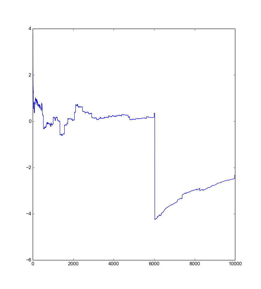

As you can see, this probably does not converge. There are some weird jumps ocurring, when you think it stops changing much. This always occurs when picking a sample which is very small or very large. In fact, this is known as Cauchy distribution and you can prove that it has no expected value. If you want to see the math, see wikipedia or a good book. This is in my opinion the easiest distribution without expected value. This characteristic is also known as fat tail.

Outro

Why is this important after all? In mathematical finance one often assumes that the prices of securities follow a brownian motion. This may work when pricing derivatives, but it is wrong in general. Some more clever approaches use a jump-diffusion process to model prices. When you are trading you need to be aware of these fat tails and cut them away. Some people try this by implementing stop losses, which may even work in theory but sucks on a practical level. You may be safer if you hedge these tails via options. But do not take my word for it.